Inspiration
Basic Abstract Spiral
  ## Data
  ab.seq <- as.data.frame(seq(from = 1,
                              to = 100,
                              by = 1))

  ab.seq$V1 <- rep(0, times = 100)

  colnames(ab.seq) <- c("ab", "V1")

  ## Plot
  ggplot() +
    geom_polygon(data = (ab.seq + 250), mapping = aes(x = 1:100, y = V1),
                 alpha = 0.5) +

    geom_point(data = (ab.seq - 150), mapping = aes(x = 1:100, y = ab)) +
    geom_point(data = (ab.seq - 100), mapping = aes(x = 1:100, y = ab)) +
    geom_point(data = (ab.seq - 50), mapping = aes(x = 1:100, y = ab)) +
    geom_point(data = (ab.seq), mapping = aes(x = 1:100, y = ab)) +
    geom_point(data = (ab.seq + 50), mapping = aes(x = 1:100, y = ab)) +
    geom_point(data = (ab.seq + 100), mapping = aes(x = 1:100, y = ab)) +
    geom_point(data = (ab.seq + 150), mapping = aes(x = 1:100, y = ab)) +
    ylim(-100, 250) +
    theme_void() +
    coord_polar()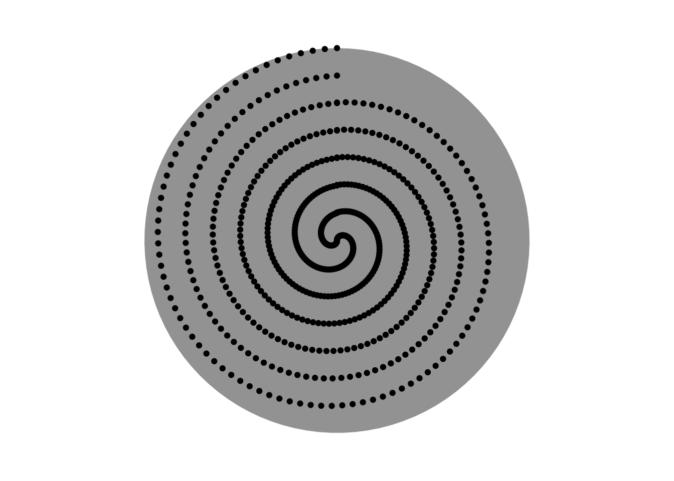
Colourful Spiral V1
## Data
  ab.seq.2 <- as.data.frame(seq(from = 0,
                                to = 99.99,
                                by = 0.01))

  ab.seq.2$ab2 <- seq(from = 99.99,
                      to = 0,
                      by = -0.01)

  ab.seq.2$col <- rep(seq(from = 1,
                          to = 5,
                          by = 1))

  ab.seq.2$V1 <- rep(0, time = 10000)

  colnames(ab.seq.2) <- c("ab", "ab2", "col", "V1")

  ggplot() +
    geom_polygon(data = (ab.seq.2 + 200),
                 mapping = aes(x = 1:10000, y = (V1)), fill = "grey") +

    geom_point(data = (ab.seq.2 - 100),
               mapping = aes(x = 1:10000, y = ab, colour = ab)) +
    geom_point(data = (ab.seq.2 - 50),
               mapping = aes(x = 1:10000, y = ab, colour = ab)) +
    geom_point(data = (ab.seq.2),
               mapping = aes(x = 1:10000, y = ab, colour = ab)) +
    geom_point(data = (ab.seq.2 + 50),
               mapping = aes(x = 1:10000, y = ab, colour = ab)) +
    geom_point(data = (ab.seq.2 + 100),
               mapping = aes(x = 1:10000, y = ab, colour = ab)) +
    geom_point(data = (ab.seq.2 + 150),
               mapping = aes(x = 1:10000, y = ab, colour = ab)) +
    geom_point(data = (ab.seq.2 + 200),
               mapping = aes(x = 1:10000, y = ab, colour = ab)) +

    geom_point(data = (ab.seq.2 - 75),
               mapping = aes(x = 1:10000, y = ab, colour = ab)) +
    geom_point(data = (ab.seq.2 - 25),
               mapping = aes(x = 1:10000, y = ab, colour = ab)) +
    geom_point(data = (ab.seq.2),
               mapping = aes(x = 1:10000, y = ab, colour = ab)) +
    geom_point(data = (ab.seq.2 + 25),
               mapping = aes(x = 1:10000, y = ab, colour = ab)) +
    geom_point(data = (ab.seq.2 + 75),
               mapping = aes(x = 1:10000, y = ab, colour = ab)) +
    geom_point(data = (ab.seq.2 + 125),
               mapping = aes(x = 1:10000, y = ab, colour = ab)) +
    geom_point(data = (ab.seq.2 + 175),
               mapping = aes(x = 1:10000, y = ab, colour = ab)) +

    ylim(0, 200) + xlim(0, 10000) +
    theme_void() +
    theme(legend.position = "none") +
    coord_polar()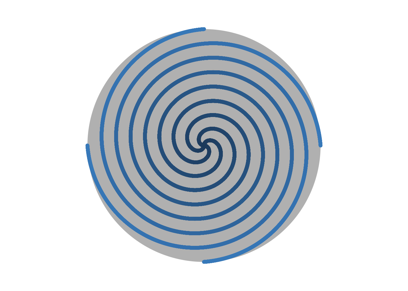
Colourful Spiral V2
## Data
  ab.seq.2 <- as.data.frame(seq(from = 0,
                                to = 99.99,
                                by = 0.01))

  ab.seq.2$ab2 <- seq(from = 99.99,
                      to = 0,
                      by = -0.01)

  ab.seq.2$col <- (rep(seq(from = 1,
                          to = 5,
                          by = 1)))

  ab.seq.2$V1 <- rep(0, time = 10000)

  colnames(ab.seq.2) <- c("ab", "ab2", "col", "V1")

  ggplot() +
    geom_polygon(data = (ab.seq.2 + 200),
                 mapping = aes(x = 1:10000, y = (V1)), fill = "lightblue") +

    geom_point(data = (ab.seq.2 - 100),
               mapping = aes(x = 1:10000, y = ab, colour = ab)) +
    geom_point(data = (ab.seq.2 - 50),
               mapping = aes(x = 1:10000, y = ab, colour = ab)) +
    geom_point(data = (ab.seq.2),
               mapping = aes(x = 1:10000, y = ab, colour = ab)) +
    geom_point(data = (ab.seq.2 + 50),
               mapping = aes(x = 1:10000, y = ab, colour = ab)) +
    geom_point(data = (ab.seq.2 + 100),
               mapping = aes(x = 1:10000, y = ab, colour = ab)) +
    geom_point(data = (ab.seq.2 + 150),
               mapping = aes(x = 1:10000, y = ab, colour = ab)) +
    geom_point(data = (ab.seq.2 + 200),
               mapping = aes(x = 1:10000, y = ab, colour = ab)) +

    geom_point(data = (ab.seq.2 - 75),
               mapping = aes(x = 1:10000, y = ab, colour = ab)) +
    geom_point(data = (ab.seq.2 - 25),
               mapping = aes(x = 1:10000, y = ab, colour = ab)) +
    geom_point(data = (ab.seq.2),
               mapping = aes(x = 1:10000, y = ab, colour = ab)) +
    geom_point(data = (ab.seq.2 + 25),
               mapping = aes(x = 1:10000, y = ab, colour = ab)) +
    geom_point(data = (ab.seq.2 + 75),
               mapping = aes(x = 1:10000, y = ab, colour = ab)) +
    geom_point(data = (ab.seq.2 + 125),
               mapping = aes(x = 1:10000, y = ab, colour = ab)) +
    geom_point(data = (ab.seq.2 + 175),
               mapping = aes(x = 1:10000, y = ab, colour = ab)) +

    scale_colour_gradient(
      low = "purple", high = "lightblue") +

    ylim(0, 200) + xlim(0, 10000) +
    theme_void() +
    theme(legend.position = "none") +
    coord_polar()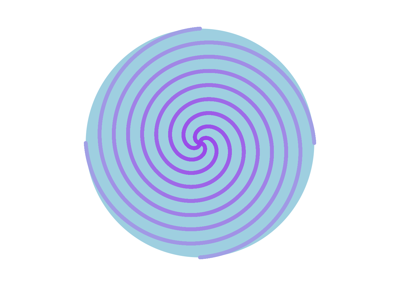
Sin Celtic Circlular Weave
fs.seq <- as.data.frame(seq(from = 1,
                              to = 51.3,
                              by = 0.25))

  fs.seq$alpha <- rep(0, times = 202)

  colnames(fs.seq) <- c("fs", "alpha")

  ggplot() +
    geom_polygon(data = fs.seq,
                 mapping = aes(x = 1:202, y = (alpha - 2))) +
    geom_polygon(data = fs.seq,
                 mapping = aes(x = 1:202, y = (alpha + 2)), alpha = 0.2) +
    geom_polygon(data = fs.seq,
                 mapping = aes(x = 1:202, y = (alpha + 4)), alpha = 0.2) +

    geom_point(data = fs.seq,
               mapping = aes(x = 1:202, y = (sin(fs) - 3))) +
    geom_point(data = fs.seq,
               mapping = aes(x = 1:202, y = (-sin(fs) - 3))) +

    geom_point(data = fs.seq,
               mapping = aes(x = 1:202, y = sin(fs))) +
    geom_point(data = fs.seq,
               mapping = aes(x = 1:202, y = -sin(fs))) +

    geom_point(data = fs.seq,
               mapping = aes(x = 1:202, y = (sin(fs) + 3))) +
    geom_point(data = fs.seq,
               mapping = aes(x = 1:202, y = (-sin(fs) + 3))) +

    ylim(-10, 10) +
    theme_void() +
coord_polar() 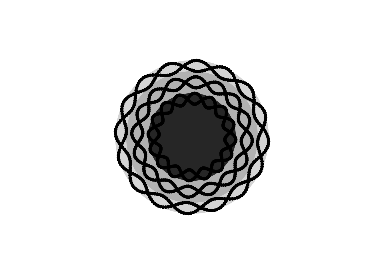
Colourful cos Celtic Circlular Weave
fs.seq <- as.data.frame(seq(from = 1,
                              to = 51.3,
                              by = 0.25))

  fs.seq$alpha <- rep(0, times = 202)

  colnames(fs.seq) <- c("fs", "alpha")

  ggplot() +
    geom_polygon(data = fs.seq,
                 mapping = aes(x = 1:202, y = (alpha - 2)),
                 alpha = 0.2, fill = "purple") +
    geom_polygon(data = fs.seq,
                 mapping = aes(x = 1:202, y = (alpha + 2)),
                 alpha = 0.2, fill = "purple") +
    geom_polygon(data = fs.seq,
                 mapping = aes(x = 1:202, y = (alpha + 4)),
                 alpha = 0.2, fill = "purple") +

    geom_point(data = fs.seq,
               mapping = aes(x = 1:202, y = ((cos(fs)-7))),
               alpha = 0.8, colour = "blue") +
    geom_point(data = fs.seq,
               mapping = aes(x = 1:202, y = ((-cos(fs)-7))),
               alpha = 0.8, colour = "red") +

    geom_point(data = fs.seq,
               mapping = aes(x = 1:202, y = (cos(fs) - 3)),
               alpha = 0.8, colour = "blue") +
    geom_point(data = fs.seq,
               mapping = aes(x = 1:202, y = (-cos(fs) - 3)),
               alpha = 0.8, colour = "red") +

    geom_point(data = fs.seq,
               mapping = aes(x = 1:202, y = cos(fs)),
               alpha = 0.5, colour = "blue") +
    geom_point(data = fs.seq,
               mapping = aes(x = 1:202, y = -cos(fs)),
               alpha = 0.5, colour = "red") +

    geom_point(data = fs.seq,
               mapping = aes(x = 1:202, y = (cos(fs) + 3)),
               alpha = 0.2, colour = "blue") +
    geom_point(data = fs.seq,
               mapping = aes(x = 1:202, y = (-cos(fs) + 3)),
               alpha = 0.2, colour = "red") +

    ylim(-10, 10) +
    theme_void() +
    coord_polar()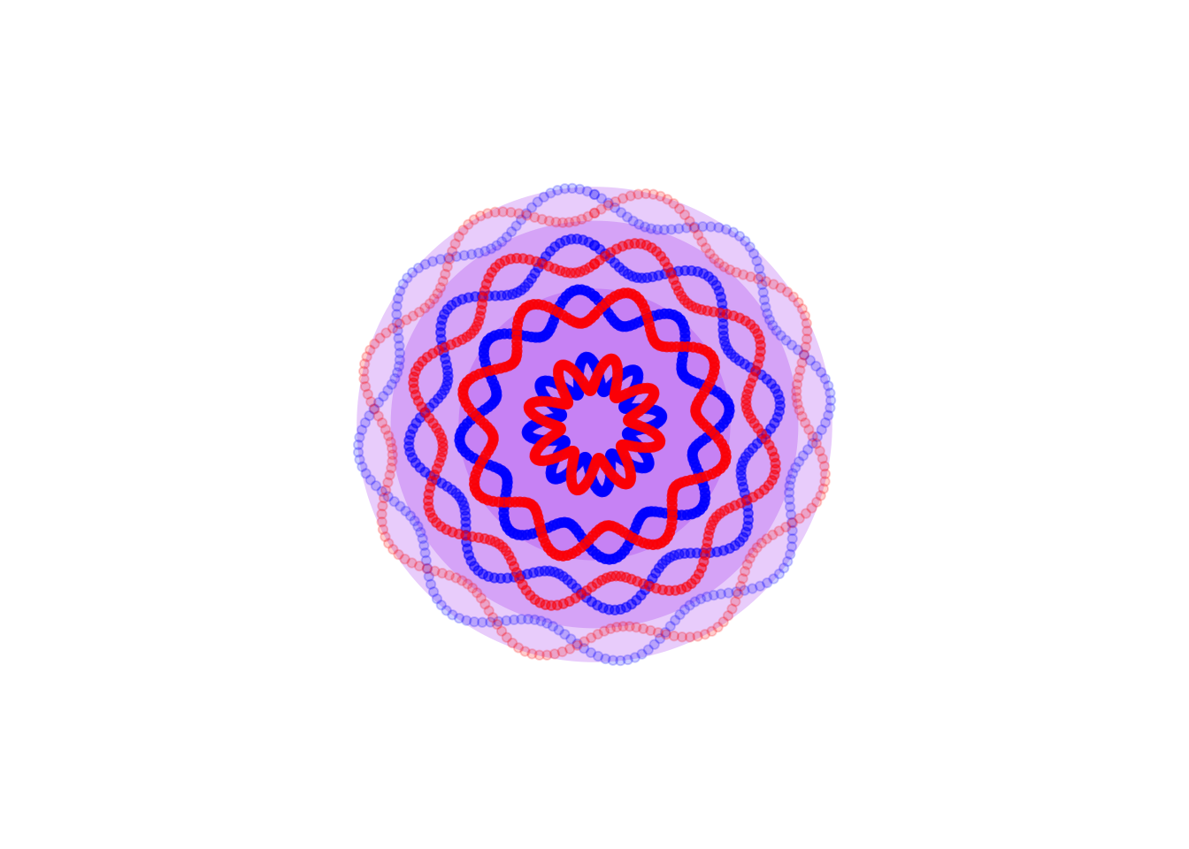
Square Weaves
kw.seq <- (seq(from = -10,
                 to = 10,
                 by = 0.05)) %>%
    expand.grid(x = ., y = .)

## Celtic Square Weave

ggplot() +
    geom_point(data = kw.seq,
              mapping = aes(x = (x + sin(y)), y = (y + cos(x))),
              alpha = 0.01, colour = "white") +
    coord_fixed() +
    theme_void() +
    theme(panel.background = element_rect(fill = "orange"))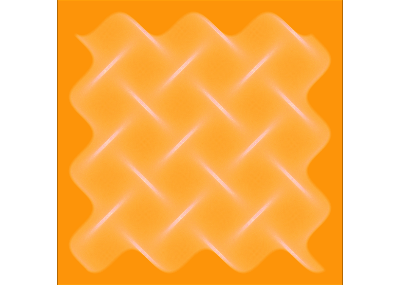
## Wave Weave

  ggplot() +
    geom_point(data = kw.seq,
               mapping = aes(x = ((x*x) + sin(y)), y = ((y*y) + cos(x))),
               alpha = 0.01, colour = "white") +
    coord_fixed() +
    theme_void() +
    theme(panel.background = element_rect(fill = "blue"))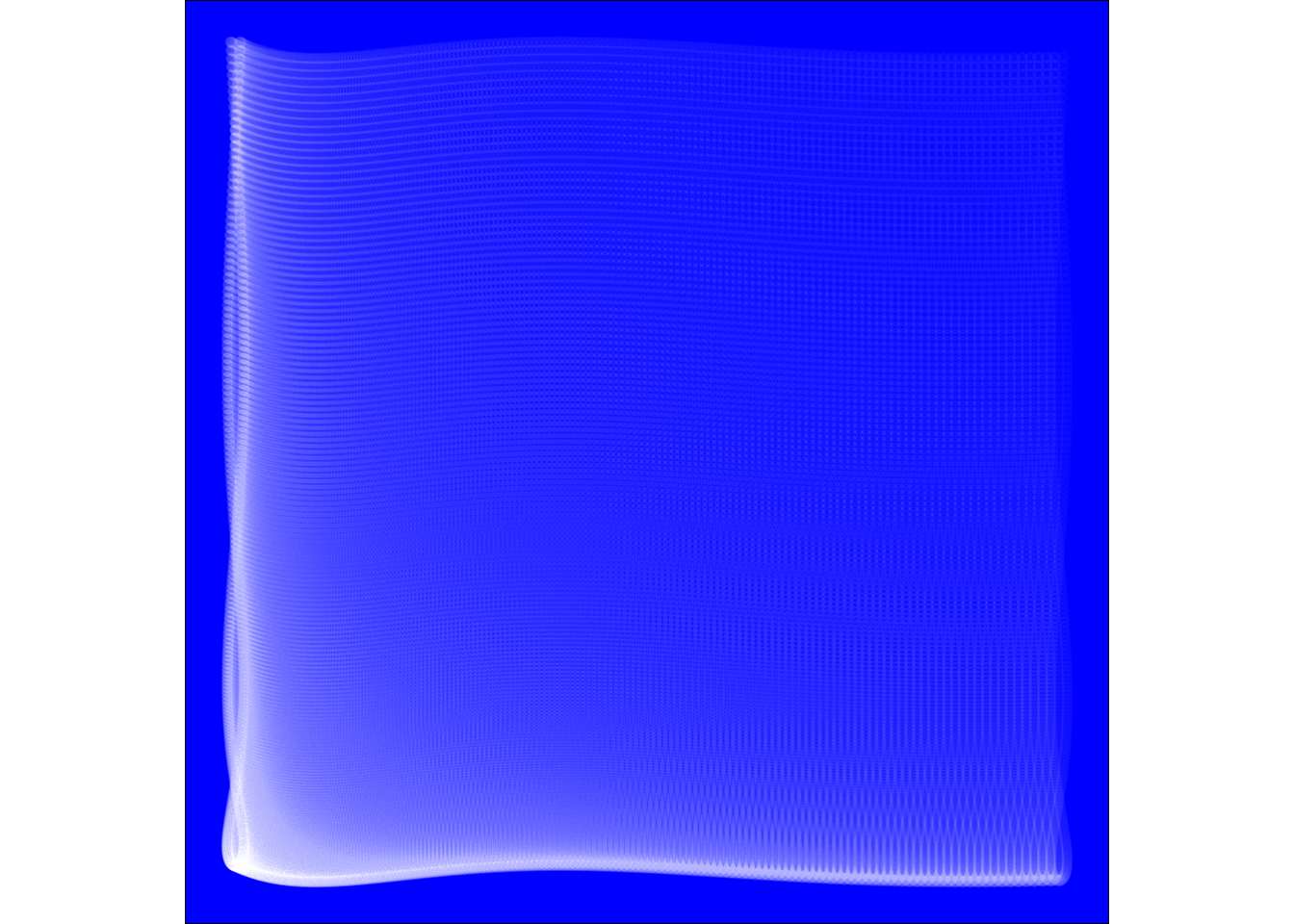
  ## Multiple Square Panel Weave
  ggplot() +
    geom_point(data = kw.seq,
               mapping = aes(x = (sin(x) + cos(x)), y = (sin(y) + cos(y))),
               alpha = 0.02, colour = "white") +
    geom_point(data = kw.seq,
               mapping = aes(x = (sin(x) + cos(x) - 2), y = (sin(y) + cos(y) - 2)),
               alpha = 0.02, colour = "blue") +
    coord_fixed() +
    theme_void() +
    theme(panel.background = element_rect(fill = "green"))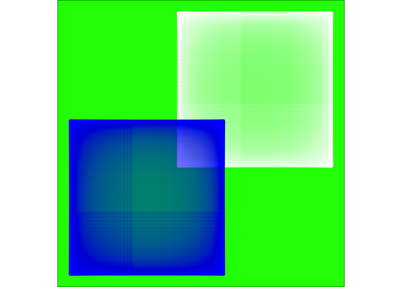
  ## Square tan Weave
  ggplot() +
    geom_point(data = kw.seq,
               mapping = aes(x = (2*x + tan(y)), y = (2*y + tan(x))),
               alpha = 0.02, colour = "white") +
    ylim(-50, 50) + xlim(-50, 50) +
    coord_fixed() +
    theme_void() +
    theme(panel.background = element_rect(fill = "green"))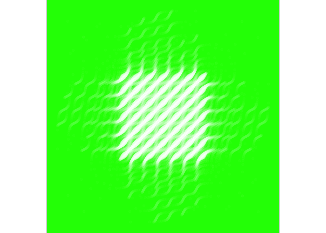
## Jellyfish

  ggplot() +
    geom_point(data = kw.seq,
               mapping = aes(x = (sqrt(x) + (sin(y))), y = (sqrt(y) + (sin(x)))),
               alpha = 0.1, colour = "blue") +
    coord_fixed() +
    theme_void() +
    theme(panel.background = element_rect(fill = "orange"))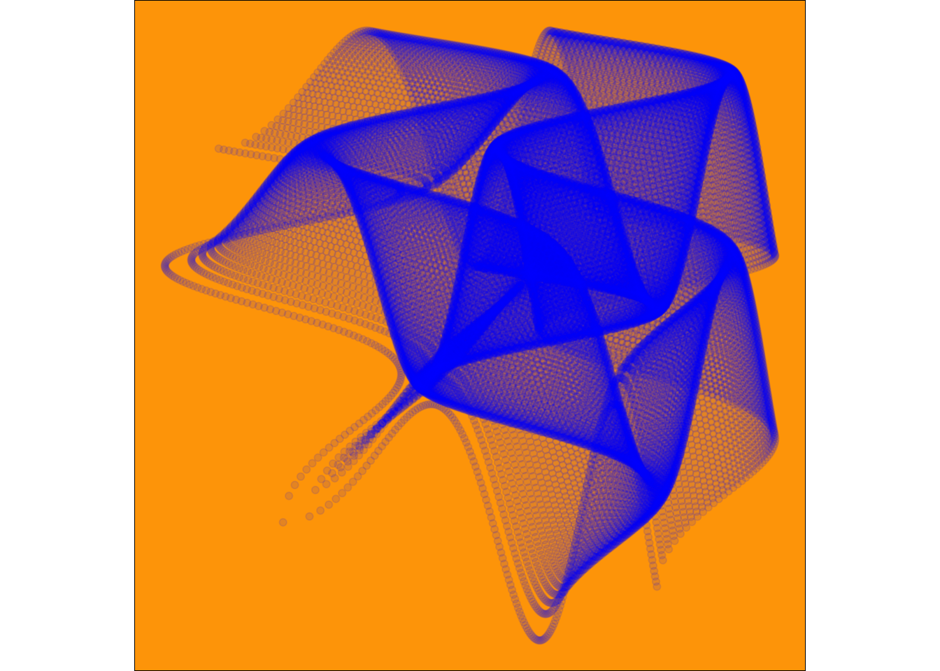
## Random Square

  ggplot() +
    geom_point(data = (kw.seq + 25),
               mapping = aes(x = (sqrt(x) + (sin(y))), y = (sqrt(y) + (sin(x)))),
               alpha = 0.02, colour = "blue") +
    coord_fixed() +
    theme_void() +
    theme(panel.background = element_rect(fill = "lightpink"))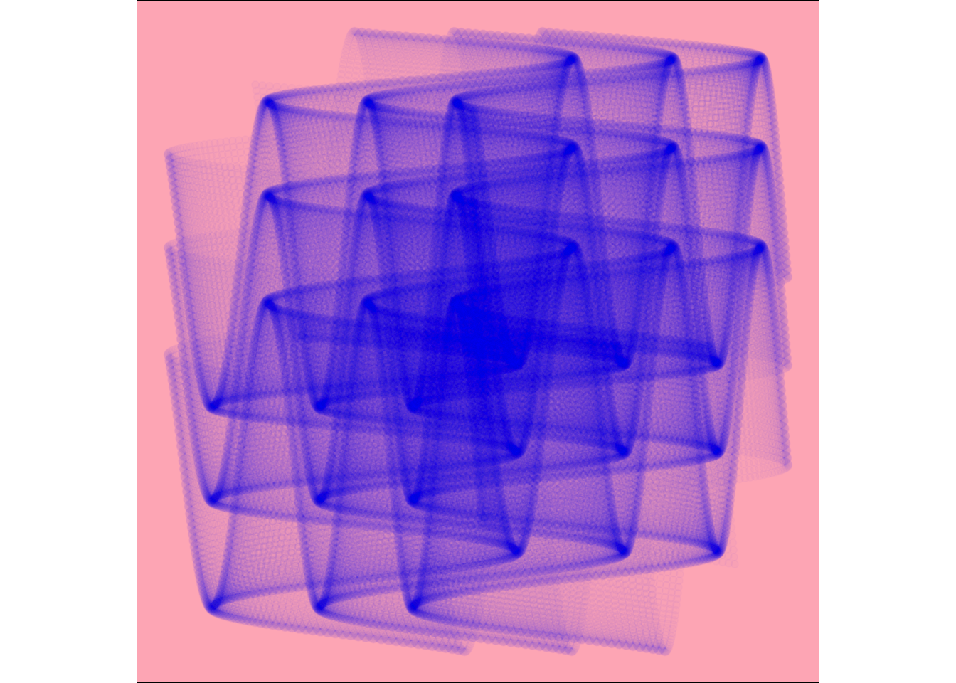
##
  ggplot() +
    geom_point(data = (kw.seq),
               mapping = aes(x = (cos(x^2)^2 + sin(y)), y = (cos(y^2)^2 + sin(x)),
                             colour = x, alpha = y)) +
    geom_point(data = (kw.seq),
               mapping = aes(x = (cos(x^2)^2 + sin(y)), y = (cos(y^2)^2 + sin(x)),
                             colour = -x, alpha = -y)) +

    coord_fixed() +
    theme_void() +
    theme(panel.background = element_rect(fill = "blue"),
          legend.position = "none")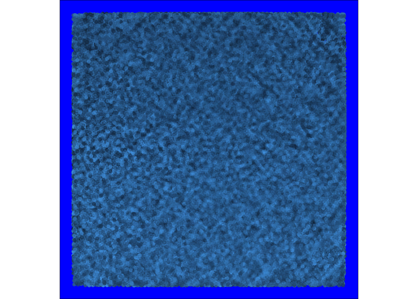
Complex Designs
Based on Fronkonstin’s blog
Summoning Cthulhu
sc.seq <- seq(from = -3,
              to = 3,
              by = 0.01) %>%
  expand.grid(x = ., y = .)

  ggplot(data = sc.seq,
         mapping = aes(x=(x^3-sin(y^2)), y=(y^3-cos(x^2)))) +
  geom_point(alpha=.1, shape=20, size=0, color="white") +
  theme_void() +
  theme(panel.background = element_rect(fill="black")) +
  coord_polar()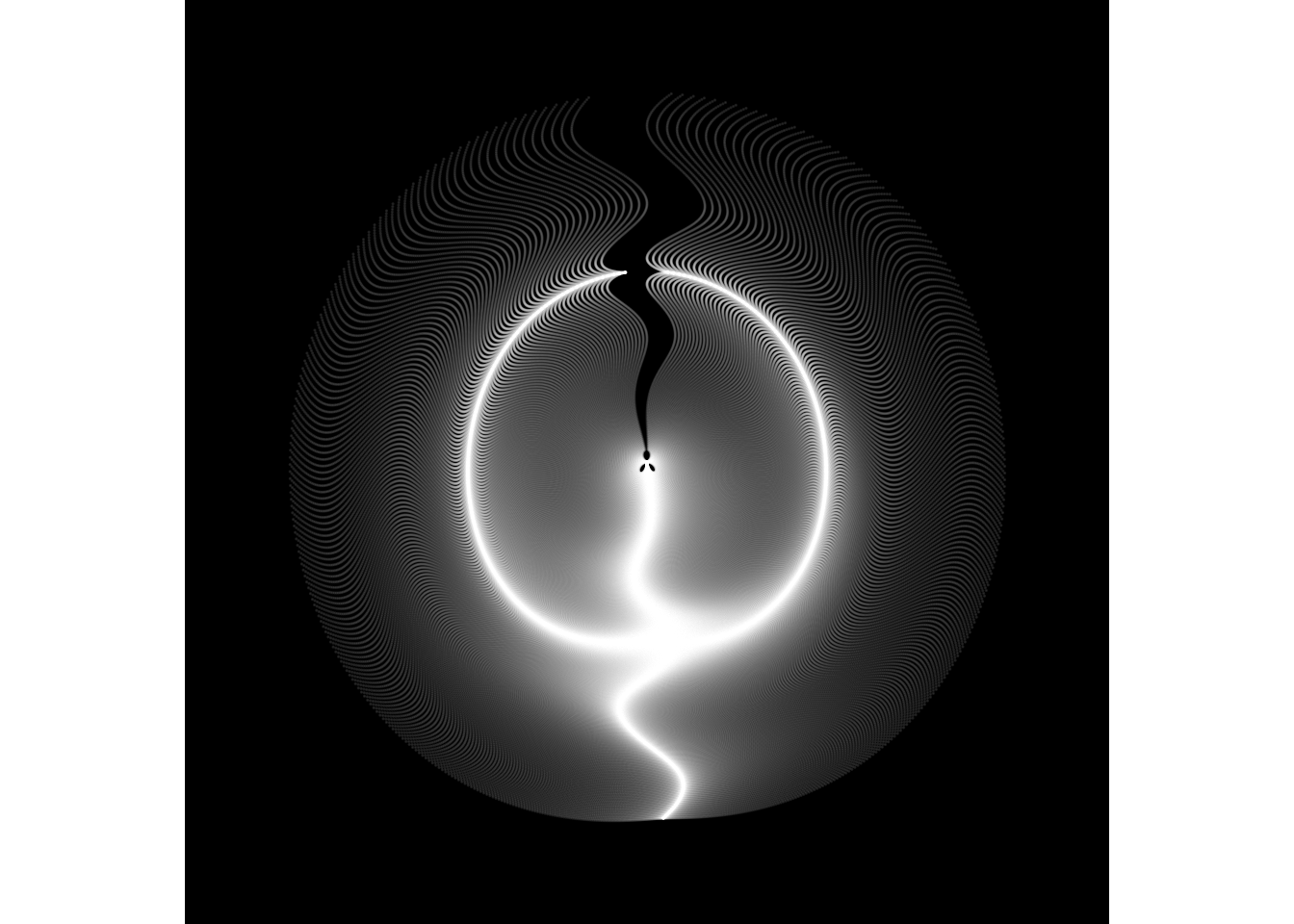
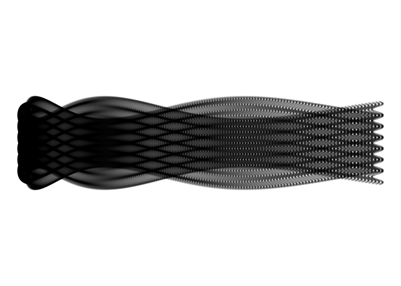
Marine Creature
mc.seq <- seq(from = -10,
              to = 10,
              by = 0.05) %>%
  expand.grid(x = ., y = .)

  ggplot(data = mc.seq,
         mapping = aes(x=(x^2+pi*cos(y)^2), y=(y+pi*sin(x)))) +
  geom_point(alpha=.1, shape=20, size=1, color="black")+
  theme_void()+coord_fixed()