Learning Materials
Getting Started with RStudio Cloud
RStudio cloud is an online service, which you will be using instead of desktop RStudio. Parts of the service (the important parts we are using) is free. You can log into this service and set up an account through your ONS or personal email.
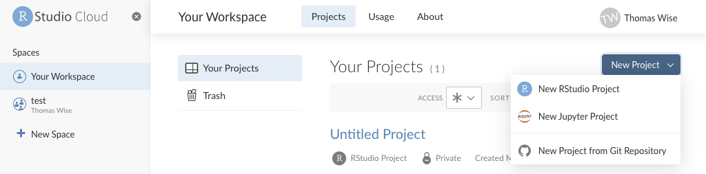
When you have logged into RStudio cloud, you can set up a new Rstudio or Jupyter project in Your Project area.
RStudio Cloud Setup
Setting up presentations in R Studio
When producing presentations in R, one of the most common setups is through Rmarkdown. Rmarkdown is a notebook interface, similar to Observable or Jupyter. And is able to integrate multiple programming language formats together to produce both static and dynamic outputs, including HTML, PDFs as well as Websites and articles.
Getting Started
Before you can open, and setup, your first presentation, you must install and load the CRAN package Rmarkdown. Although we will only use a limited number of functions directly from this package, this provides the infrastructure required in R Studio in order to open and setup presentations.
To install ‘Rmarkdown’ run the following:
install.packages("rmarkdown")
library(rmarkdown)
Please note, it is advised you do not restart R prior to installing the package, as it will otherwise loop the same error message! If you don’t get this message, don’t panic!
Once installed, restart your R Studio. This will unlock access to additional addins and procedures required for this session.
Once restarted, open an empty project file, and access: File -> New File -> R Markdown.
This will open up the following window and select Document.
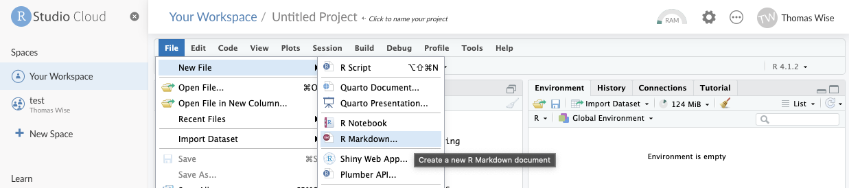
If you select OK rather than Create Empty Document this will generate a demonstrative presentation in your selected default output format.
As we will be working with PDF formats also, ensure you have also downloaded the relevant TeX program (if possible). For Windows here, for Macs here, or Linux here.
Knitting your first document
Before we dive deeper into the syntax and in depth elements of these procedures, ensure you can save and knit your document successfully. For this select the Knit button, specify the location to save. This should produce a pop-out window, containing the HTML file of your presentation.
At this point, if you are simply setting up your R Studio for our live session, you can stop here. However if you are completing this independently we will dive further into the finer points of R Markdown documents.
Standard R markdown Syntax for Presentations
As a document compiler, R markdown is underwritten by the language LaTeX and through TeX allows the production of files. In mainstream academia, LaTeX processers are incredibly common, due to its free nature, as well as flexibility across the publication of scientific documents.
Since R markdown is underwritten by LaTeX and compiled through TeX, there is a large amount of syntax which can be used between different R markdown document types (presentations, reports and websites). However, there is also syntax specific for presentations. We will first cover the syntax specific for presentations, before covering some useful universal syntax. A summary of this syntax can be found under Cheat sheets & Helpful Guides.
Overall Metadata: General
The header in an R markdown document, defines the YAML metadata, such as outlining the:
title:- Title of the documentsubtitle:- Secondary/Sub title of the documentoutput:- Output type (html, pdf, etc)date:- Listed dateauthor:- Document authorsemail:- Author emailsfontsize:- Font Sizelinkcolor,urlcolor&citecolor: colour for links, urls and cites
Additionally, different file formats also have additional parameters which can be defined:
Overall Metadata: PDF
Add a Table of Contents:
toc: trueIndicate Table of Content Depth:
toc_depth: 2Indicate section numbers:
number_sections: trueSpecify figures
fig_width,fig_heightandfig_caption
Data frames
df_print: kable(this uses the kable package)
Overall Metadata: HTML
Add a Table of Contents:
toc: trueIndicate Table of Content Depth:
toc_depth: 2Indicate section numbers:
number_sections: trueFloating Table of Content
number_sections: trueDoes the Table of Content collapse:
collapsed: trueAnimated Page scrolles:
smooth_scroll: trueSpecify figures
fig_width,fig_heightandfig_caption
Tabbed sections (inline): ## Section Head {.tabset}
Data frames
df_print: kable(uses the kable package)df_print: tibble(uses the tibble package)df_print: paged(uses the rmarkdown package)
Themes:
theme:- from: bootswatch.comunited,Cosmo,Darkly
Highlight:
highlight:default,tango,espresso
Code Folding:
code_folding: hide
Document Syntax, Code Chunks & Equations
Document Syntax
When writing any length of text, LaTeX syntax can be deployed:
Bullet Points:
-Block Quotes:
> -Numbered Lists:
1.,2.Italic Text:
* *or_ _Bold Text:
** **or__ __Strike Through:
~~ ~~Superscript:
^ ^Subscript:
~ ~Indent Text
|Footnotes:
^[]In text links:
[](<>)In text image:
TeX Formula:
$ $
Code Chunks
In a normal document, it is possible to either display code, provide results or data visualizations with relative ease. Since R markdown, similar to other notebooks, uses code chunks to contain their code.
Within R markdown, code chunks delimiters are written as such:
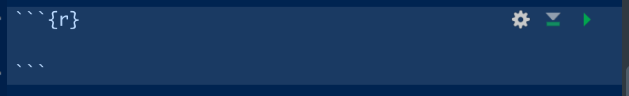
R Markdown Code Chunk
These code chunks act in the same way as regular code script. But can be customized with the knitr options, with the arguments set within the { }. Typically, there are five commonly used arguments (although more exist).
- include = FALSE - prevents code and results from appearing in the finished file, code is still run.
- echo = FALSE - prevents code, but not results from appearing in the finished file.
- message = FALSE - prevents messages, generated by code from appearing in the finished file.
- warning = FALSE - prevents warnings, generated by code from appearing in the finished file.
- fig.cap = “…” - adds a caption to a graphical result.
- fig.height / fig.width = … - Defines figure height / width.
When using these code chunks within your presentation, to display data visualizations, it is important to use a combination. Most typically, this includes: echo = FALSE, message = FALSE, warning = FALSE in addition to figure parameters.
Equations in Documents
Equations are written using LaTeX syntax more precisely
- Inline equations are between dollar signs:
$....$ - Display style equations are between double dollar signs:
$$....$$
These can be combined with LaTeX styling:
- Greek Lettering:
\Thetafor capital theta - To power of:
^{}
A more detail manual of this can be found online in Mathematics in R Markdown by R. Pruim and R Markdown for Scientists by N. Tierney
References & Citations in Documents
You can setup a referencing system in any document using the following steps:
- Create BibTeX database, or .bib plain-text file (save a .txt file with extension .bib)
- Add
bibliography: references.bibfile. - Populate BibTeX database with entries.
- Reference in line with
[@referenceuniquekey](aka the first line) - The bibliography will automatically be populated at the bottom of your document
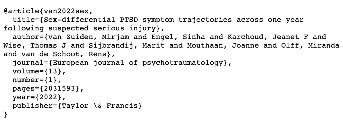
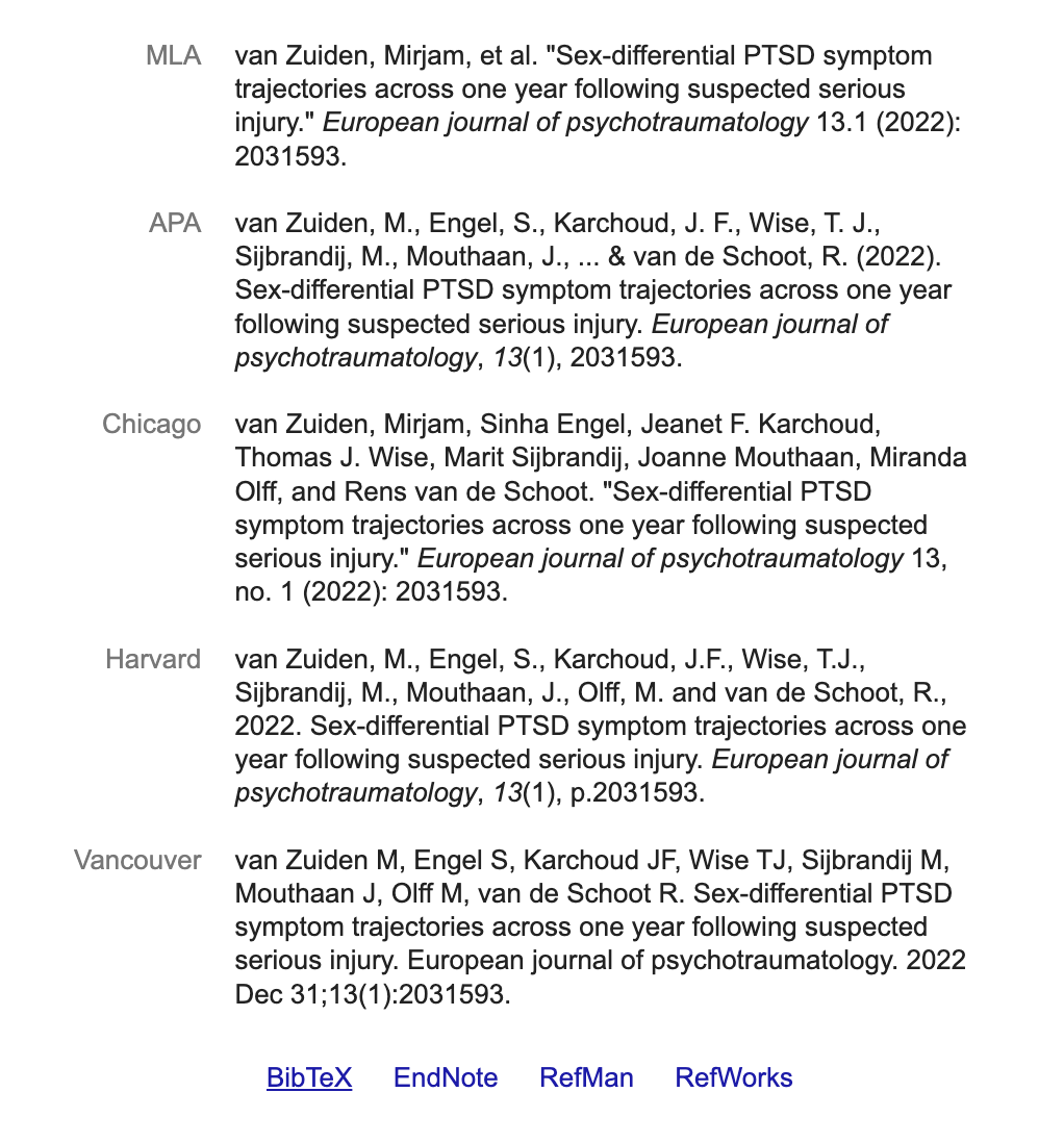
BibTeX Style Reference
To get this reference format, simply select BibTex on the Google Scholar cite menu
Google Scholar Cite Page Reference
By Default: pandoc-citeproc uses Chicago author-date format. To change this, specify a CSL (Citation Style Language) file in the csl: metadata field.
Download these from journals directly, or The Zotero Style Repository (https://www.zotero.org/styles)
Exporting and using documents
Exporting and using presentations, as discussed above, is completed through knitting the presentation via the Knitr package.
Documents can be knit to various formats including HTML, PDF or ODS.
Once saved, these can then be used as regular document or file from your file directory.
Additionally, there are several alternatives to Rmarkdown including:
- Overleaf (premium for non-students)
- TeXmaker
- Kile LaTex Editor